day 27 Activation Functions

Activation Functions.

import numpy as np
import matplotlib.pyplot as plt
from PIL import Image
from itertools import product
import tensorflow as tf

tf.random.set_seed(7879)

print('Ready to activate?⤴')

Ready to activate?⤴

activation functions

Activation functions increases the expressivity or the representation capacity of the model.

perceptron

우리가 알고 있는 딥러닝 모델은 보통 여러 개의 층으로 이루어져 있습니다. 그중에 하나의 층을 가져와 다시 쪼갠다면 보통 ‘노드’라고 불리는 것으로 쪼개지게 되는데, 이것이 바로 퍼셉트론(Perceptron)입니다.

합쳐진 신호는 세포체에서 신호를 처리하는 방식과 비슷하게 적절한 활성화 함수(activation function) ff 를 거쳐 출력이 결정됩니다.

any downwards flow that is over the certain value is expressed while others not. Activations functions are often called transfer functions as well. and depending on the way it is expressed, it can be a

• 선형 활성화 함수(Linear activation function)

• 비선형 활성화 함수(Non-linear activation function)

linear activation function

def binary_step(x, threshold=0): 
# threshold가 있는 함수를 쓰면 꼭 defualt 값을 설정해주세요
    return 0 if x<threshold else 1

import matplotlib.pyplot as plt
from PIL import Image
import numpy as np

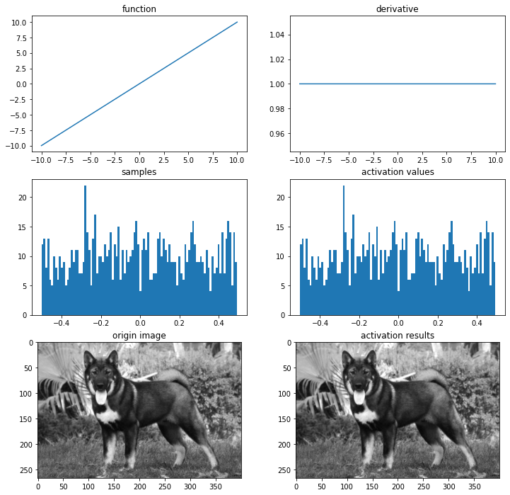
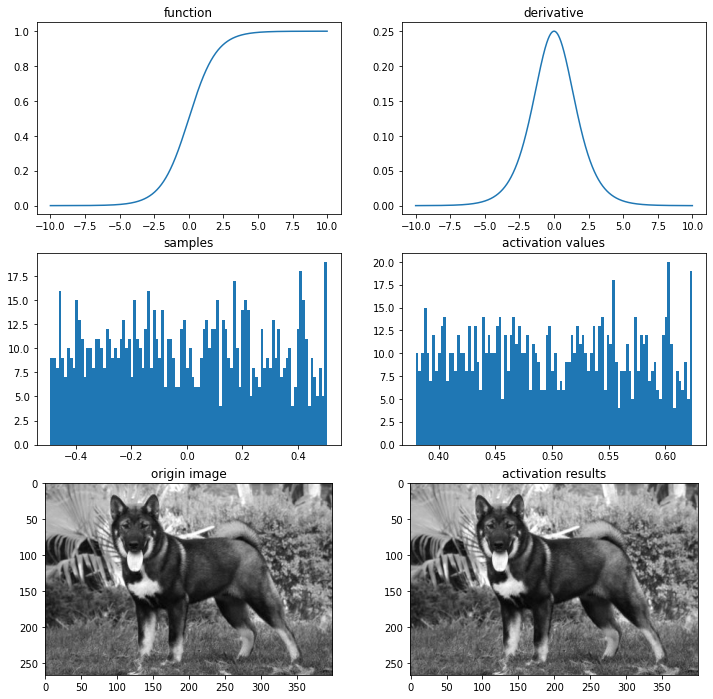
def plot_and_visulize(image_url, function, derivative=False):
    X = [-10 + x/100 for x in range(2000)]
    y = [function(y) for y in X]
    
    plt.figure(figsize=(12,12))
    
    # 함수 그래프
    plt.subplot(3,2,1)
    plt.title('function')
    plt.plot(X,y)
    
    # 함수의 미분 그래프
    plt.subplot(3,2,2)
    plt.title('derivative')
    if derivative:
        dev_y = [derivative(y) for y in X]
        plt.plot(X,dev_y)
    
    # 무작위 샘플들 분포
    samples = np.random.rand(1000)
    samples -= np.mean(samples)
    plt.subplot(3,2,3)
    plt.title('samples')
    plt.hist(samples,100)
    
    # 활성화 함수를 통과한 샘플들 분포
    act_values = [function(y) for y in samples]
    plt.subplot(3,2,4)
    plt.title('activation values')
    plt.hist(act_values,100)
    
    # 원본 이미지
    image = np.array(Image.open(image_url), dtype=np.float64)[:,:,0]/255. # 구분을 위해 gray-scale해서 확인
    image -= np.median(image)
    plt.subplot(3,2,5)
    plt.title('origin image')
    plt.imshow(image, cmap='gray')
    
    # 활성화 함수를 통과한 이미지
    activation_image = np.zeros(image.shape)
    h, w = image.shape
    for i in range(w):
        for j in range(h):
            activation_image[j][i] += function(image[j][i])
    plt.subplot(3,2,6)
    plt.title('activation results')
    plt.imshow(activation_image, cmap='gray')
    
    return plt

import os
img_path = os.getenv('HOME')+'/aiffel/activation/jindo_dog.jpg'
ax = plot_and_visulize(img_path, binary_step)
ax.show()

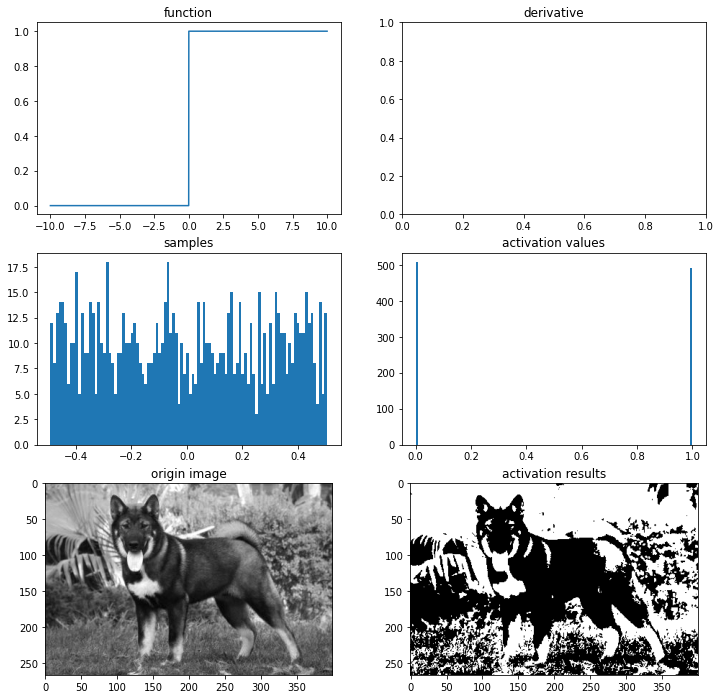
이진 계단 함수의 치역(range)은 00,11 (00과 11만 나온다는 뜻)이 됩니다.

이진 계단 함수는 단층 퍼셉트론(single layer perceptrons)라는 초기의 신경망에서 자주 사용되었습니다.

# 퍼셉트론
class Perceptron(object):
    def __init__(self, input_size, activation_ftn, threshold=0, learning_rate=0.01):
        self.weights = np.random.randn(input_size)
        self.bias = np.random.randn(1)
        self.activation_ftn = np.vectorize(activation_ftn)
        self.learning_rate = learning_rate
        self.threshold = threshold

    def train(self, training_inputs, labels, epochs=100, verbose=1):
        '''
        verbose : 0-매 에포크 결과 출력, 
                  1-마지막 결과만 출력 
        '''
        for epoch in range(epochs):
            for inputs, label in zip(training_inputs, labels):
                prediction = self.__call__(inputs)
                self.weights += self.learning_rate * (label - prediction) * inputs
                self.bias += self.learning_rate * (label - prediction)
            if verbose == 1:
                pred = self.__call__(training_inputs)
                accuracy = np.sum(pred==labels)/len(pred)
                print(f'{epoch}th epoch, accuracy : {accuracy}')
        if verbose == 0:
            pred = self.__call__(training_inputs)
            accuracy = np.sum(pred==labels)/len(pred)
            print(f'{epoch}th epoch, accuracy : {accuracy}')
    
    def get_weights(self):
        return self.weights, self.bias
                
    def __call__(self, inputs):
        summation = np.dot(inputs, self.weights) + self.bias
        return self.activation_ftn(summation, self.threshold)

def scatter_plot(plt, X, y, threshold = 0, three_d=False):
    ax = plt
    if not three_d:
        area1 = np.ma.masked_where(y <= threshold, y)
        area2 = np.ma.masked_where(y > threshold, y+1)
        ax.scatter(X[:,0], X[:,1], s = area1*10, label='True')
        ax.scatter(X[:,0], X[:,1], s = area2*10, label='False')
        ax.legend()
    else:
        area1 = np.ma.masked_where(y <= threshold, y)
        area2 = np.ma.masked_where(y > threshold, y+1)
        ax.scatter(X[:,0], X[:,1], y-threshold, s = area1, label='True')
        ax.scatter(X[:,0], X[:,1], y-threshold, s = area2, label='False')
        ax.scatter(X[:,0], X[:,1], 0, s = 0.05, label='zero', c='gray')
        ax.legend()
    return ax

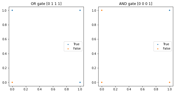
# AND gate, OR gate
X = np.array([[0,0], [1,0], [0,1], [1,1]])

plt.figure(figsize=(10,5))
# OR gate
or_y = np.array([x1 | x2 for x1,x2 in X])
ax1 = plt.subplot(1,2,1)
ax1.set_title('OR gate ' + str(or_y))
ax1 = scatter_plot(ax1, X, or_y)

# AND gate
and_y = np.array([x1 & x2 for x1,x2 in X])
ax2 = plt.subplot(1,2,2)
ax2.set_title('AND gate ' + str(and_y))
ax2 = scatter_plot(ax2, X, and_y)

plt.show()

# OR gate
or_p = Perceptron(input_size=2, activation_ftn=binary_step)
or_p.train(X, or_y, epochs=1000, verbose=0)
print(or_p.get_weights()) # 가중치와 편향값은 훈련마다 달라질 수 있습니다.

# AND gate
and_p = Perceptron(input_size=2, activation_ftn=binary_step)
and_p.train(X, and_y, epochs=1000, verbose=0)
print(and_p.get_weights()) # 가중치와 편향값은 훈련마다 달라질 수 있습니다.

999th epoch, accuracy : 1.0
(array([0.45831892, 1.40860268]), array([-0.44386656]))
999th epoch, accuracy : 1.0
(array([0.00154557, 0.66992457]), array([-0.67095938]))

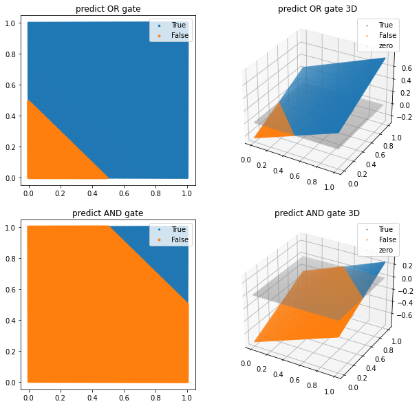
from itertools import product

# 그래프로 그려보기
test_X = np.array([[x/100,y/100] for (x,y) in product(range(101),range(101))])
pred_or_y = or_p(test_X)
pred_and_y = and_p(test_X)

plt.figure(figsize=(10,10))
ax1 = plt.subplot(2,2,1)
ax1.set_title('predict OR gate')
ax1 = scatter_plot(ax1, test_X, pred_or_y)

ax2 = plt.subplot(2,2,2, projection='3d')
ax2.set_title('predict OR gate 3D')
ax2 = scatter_plot(ax2, test_X, pred_or_y, three_d=True)

ax3 = plt.subplot(2,2,3)
ax3.set_title('predict AND gate')
ax3 = scatter_plot(ax3, test_X, pred_and_y)

ax4 = plt.subplot(2,2,4, projection='3d')
ax4.set_title('predict AND gate 3D')
ax4 = scatter_plot(ax4, test_X, pred_and_y, three_d=True)

plt.show()

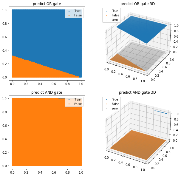
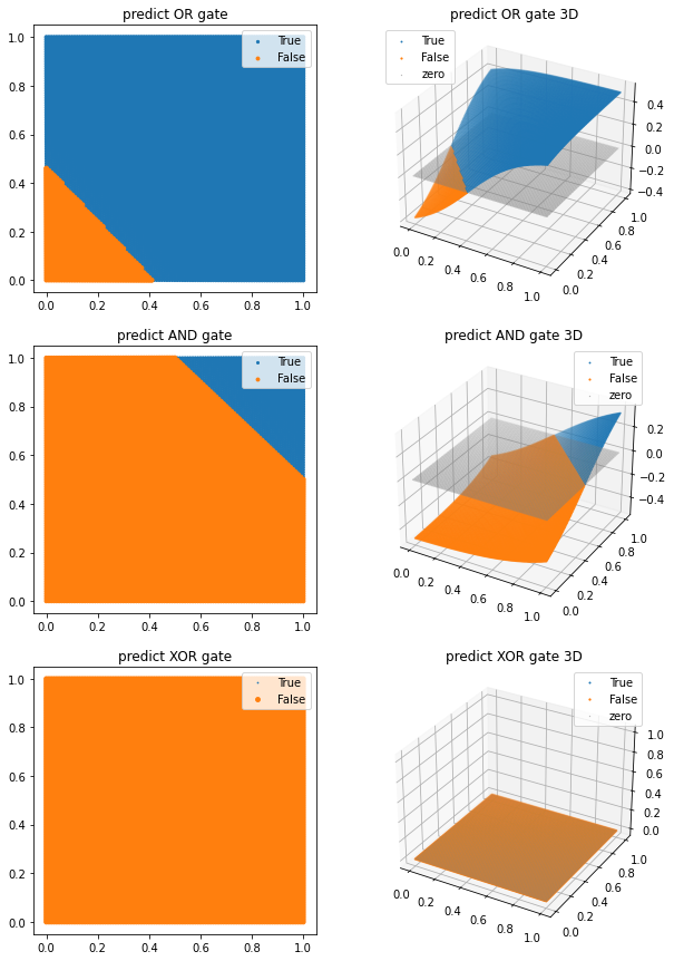
그럼 우리의 단층 퍼셉트론 모델의 추론 결과를 그래프로 그려 보겠습니다. 위에서 그려보았던 그래프가 4개의 점으로 표시된 것에 비해, 아래 그려질 그래프는 x, y축를 100등분한 결과를 모델에 대입하여 True와 False의 경계선이 선형적으로 드러나도록 그려질 것입니다. 위에서 언급한 것처럼 퍼셉트론이 하나의 선으로 구분할 수 있는 문제를 풀 수 있다 는 것을 시각적으로 확인하기 위해서입니다.

limitations

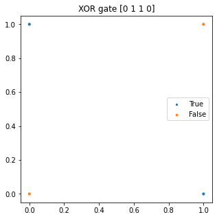
# XOR gate
threshold = 0
X = np.array([[0,0], [1,0], [0,1], [1,1]])

plt.figure(figsize=(5,5))
xor_y = np.array([x1 ^ x2 for x1,x2 in X])
plt.title('XOR gate '+ str(xor_y))
plt = scatter_plot(plt, X, xor_y)
plt.show()

# XOR gate가 풀릴까?
xor_p = Perceptron(input_size=2, activation_ftn=binary_step, threshold=threshold)
xor_p.train(X, xor_y, epochs=1000, verbose=0)
print(xor_p.get_weights())

# 그래프로 그려보기
test_X = np.array([[x/100,y/100] for (x,y) in product(range(101),range(101))])
pred_xor_y = xor_p(test_X)

plt.figure(figsize=(10,5))
ax1 = plt.subplot(1,2,1)
ax1.set_title('predict XOR gate?')
ax1 = scatter_plot(ax1, test_X, pred_xor_y)

ax2 = plt.subplot(1,2,2, projection='3d')
ax2.set_title('predict XOR gate 3D?')
ax2 = scatter_plot(ax2, test_X, pred_xor_y, three_d=True)

plt.show()

999th epoch, accuracy : 0.25
(array([-0.01407581, -0.01860697]), array([0.0094996]))

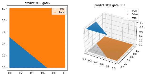
떤가요? 이번에 나온 accuracy는 무려…. 0.25밖에 안됩니다. 왜 그럴까요?

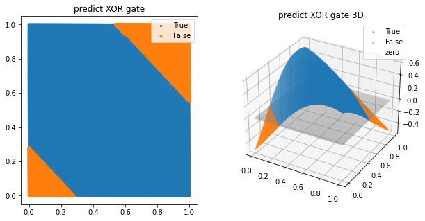
단층 퍼셉트론은 이 XOR gate를 구현할 수 없습니다. 왜냐하면 XOR gate의 진릿값 그래프를 하나의 선으로 구분을 할 수 없기 때문입니다. 하지만 이를 해결할 수 있는 방법이 있습니다. 바로 여러 층을 쌓는 것입니다. 이렇게 여러 층을 쌓은 모델을 다층 퍼셉트론(multi-layer perceptron, MLP) 이라고 합니다.

이처럼 층만 쌓으면 이진 계단 함수를 사용한 모델은 비선형적 데이터도 예측할 수 있습니다. 하지만 이진 계단 함수는 몇 가지 큰 단점이 있습니다.

바로 역전파 알고리즘(backpropagation algorithm)을 사용하지 못하는 것입니다. 이진 계단 함수는 00에서는 미분이 안 될 뿐더러 00인 부분을 제외하고 미분을 한다고 해도 미분값이 전부 00이 나옵니다. 때문에 역전파에서 가중치들이 업데이트되지 않습니다.

또한 다중 출력은 할 수 없다는 단점이 있습니다. 이진 계단 함수는 출력을 11 또는 00으로 밖에 주지 못하기 때문에 다양한 클래스를 구분해야 하는 문제는 해결할 수 없습니다.

linear activation functions

import os
img_path = os.getenv('HOME')+'/aiffel/activation/jindo_dog.jpg'

# 선형 함수
def linear(x):
    return x

def dev_linear(x):
    return 1

# 시각화
ax = plot_and_visulize(img_path, linear, dev_linear)
ax.show()

# AND gate, OR gate
threshold = 0
X = np.array([[0,0], [1,0], [0,1], [1,1]])

plt.figure(figsize=(10,5))
# OR gate
or_y = np.array([x1 | x2 for x1,x2 in X])
ax1 = plt.subplot(1,2,1)
ax1.set_title('OR gate ' + str(or_y))
ax1 = scatter_plot(ax1, X, or_y)

# AND gate
and_y = np.array([x1 & x2 for x1,x2 in X])
ax2 = plt.subplot(1,2,2)
ax2.set_title('AND gate ' + str(and_y))
ax2 = scatter_plot(ax2, X, and_y)

plt.show()

import tensorflow as tf

# OR gate model
or_linear_model = tf.keras.Sequential([
    tf.keras.layers.Input(shape=(2,), dtype='float64'),
    tf.keras.layers.Dense(1, activation='linear')
])
or_linear_model.compile(loss='mse', optimizer=tf.keras.optimizers.Adam(learning_rate=0.01), metrics=['accuracy'])
or_linear_model.summary()

# AND gate model
and_linear_model = tf.keras.Sequential([
    tf.keras.layers.Input(shape=(2,), dtype='float64'),
    tf.keras.layers.Dense(1, activation='linear')
])
and_linear_model.compile(loss='mse', optimizer=tf.keras.optimizers.Adam(learning_rate=0.01), metrics=['accuracy'])
and_linear_model.summary()

Model: "sequential_3"
_________________________________________________________________
Layer (type)                 Output Shape              Param #   
=================================================================
dense_3 (Dense)              (None, 1)                 3         
=================================================================
Total params: 3
Trainable params: 3
Non-trainable params: 0
_________________________________________________________________
Model: "sequential_4"
_________________________________________________________________
Layer (type)                 Output Shape              Param #   
=================================================================
dense_4 (Dense)              (None, 1)                 3         
=================================================================
Total params: 3
Trainable params: 3
Non-trainable params: 0
_________________________________________________________________

or_linear_model.fit(X, or_y, epochs=1000, verbose=0)
and_linear_model.fit(X, and_y, epochs=1000, verbose=0)
print('done')

done

# 그래프로 그려보기
test_X = np.array([[x/100,y/100] for (x,y) in product(range(101),range(101))])
pred_or_y = or_linear_model(test_X)
pred_and_y = and_linear_model(test_X)

plt.figure(figsize=(10,10))
ax1 = plt.subplot(2,2,1)
ax1.set_title('predict OR gate')
ax1 = scatter_plot(ax1, test_X, pred_or_y, threshold=0.5)

ax2 = plt.subplot(2,2,2, projection='3d')
ax2.set_title('predict OR gate 3D')
ax2 = scatter_plot(ax2, test_X, pred_or_y, threshold=0.5, three_d=True)

ax3 = plt.subplot(2,2,3)
ax3.set_title('predict AND gate')
ax3 = scatter_plot(ax3, test_X, pred_and_y, threshold=0.5)

ax4 = plt.subplot(2,2,4, projection='3d')
ax4.set_title('predict AND gate 3D')
ax4 = scatter_plot(ax4, test_X, pred_and_y, threshold=0.5, three_d=True)

plt.show()

# XOR gate
xor_linear_model = tf.keras.Sequential([
    tf.keras.layers.Input(shape=(2,), dtype='float64'),
    tf.keras.layers.Dense(1, activation='linear')
])
xor_linear_model.compile(loss='mse', optimizer=tf.keras.optimizers.Adam(learning_rate=0.01), metrics=['accuracy'])
xor_linear_model.fit(X, xor_y, epochs=1000, verbose=0)

# 그래프로 그려보기
test_X = np.array([[x/100,y/100] for (x,y) in product(range(101),range(101))])
pred_xor_y = xor_linear_model(test_X)

plt.figure(figsize=(10,5))
ax1 = plt.subplot(1,2,1)
ax1.set_title('predict XOR gate')
ax1 = scatter_plot(ax1, test_X, pred_xor_y, threshold=0.5)

ax2 = plt.subplot(1,2,2, projection='3d')
ax2.set_title('predict XOR gate 3D')
ax2 = scatter_plot(ax2, test_X, pred_xor_y, threshold=0.5, three_d=True)

plt.show()

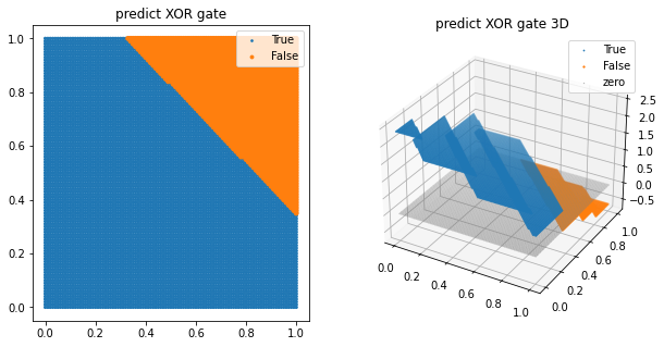
그럼 이 모델로 XOR gate를 구현할 수 있을까요? 정답은 ‘불가능하다’ 입니다. 마찬가지로 선 하나로는 나눌 수 없기 때문입니다.선형 활성화 함수의 한계는 명확합니다. 바로 모델에 선형 활성화 함수를 사용한다면 비선형적 특성을 지닌 데이터를 예측하지 못 한다는 것입니다. 이 부분은 조금 전에 자세히 다루었기 때문에 넘어가도록 하겠습니다.

non-linear activation functions

sigmoid / logistic

import os
img_path = os.getenv('HOME')+'/aiffel/activation/jindo_dog.jpg'

# 시그모이드 함수
def sigmoid(x):
    return 1/(1+np.exp(-x).astype(np.float64))

def dev_sigmoid(x):
    return sigmoid(x)*(1-sigmoid(x))

# 시각화
ax = plot_and_visulize(img_path, sigmoid, dev_sigmoid)
ax.show()

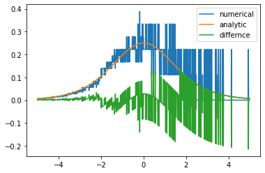
# 수치 미분
def num_derivative(x, function):
    h = 1e-15 # 이 값을 바꾸어 가며 그래프를 확인해 보세요
    numerator = function(x+h)-function(x)
    return numerator/h

# 두 그래프의 차이
diff_X = [-5+x/100 for x in range(1001)]
dev_y = np.array([dev_sigmoid(x) for x in diff_X])
num_dev_y = np.array([num_derivative(x, sigmoid) for x in diff_X])

diff_y = dev_y - num_dev_y
plt.plot(diff_X, num_dev_y, label='numerical')
plt.plot(diff_X, dev_y, label='analytic')
plt.plot(diff_X, diff_y, label='differnce')
plt.legend()

plt.show()

disadvantages of sigmoid

시그모이드 함수는 00 또는 11에서 포화(saturate) 됩니다. 이것을 ‘그래디언트를 죽인다(kill the gradient)’ 라고 표현합니다. 극단적인 예로 만약 어떤 모델의 초기 가중치 값들을 아주 크게 잡아 포화상태를 만들면 역전파 때 그래디언트가 죽기 때문에 아무리 많이 에포크를 돌려도 훈련이 거의 되지 않습니다.

시그모이드 함수의 출력은 0이 중심(zero-centered)이 아닙니다. 여기서 발생하는 문제는 훈련의 시간이 오래걸리게 된다는 것입니다.

# OR gate
or_sigmoid_model = tf.keras.Sequential([
    tf.keras.layers.Input(shape=(2,)),
    tf.keras.layers.Dense(1, activation='sigmoid')
])
or_sigmoid_model.compile(loss='mse', optimizer=tf.keras.optimizers.Adam(learning_rate=0.01), metrics=['accuracy'])
or_sigmoid_model.fit(X, or_y, epochs=1000, verbose=0)

# AND gate
and_sigmoid_model = tf.keras.Sequential([
    tf.keras.layers.Input(shape=(2,)),
    tf.keras.layers.Dense(1, activation='sigmoid')
])
and_sigmoid_model.compile(loss='mse', optimizer=tf.keras.optimizers.Adam(learning_rate=0.01), metrics=['accuracy'])
and_sigmoid_model.fit(X, and_y, epochs=1000, verbose=0)

# XOR gate
xor_sigmoid_model = tf.keras.Sequential([
    tf.keras.layers.Input(shape=(2,)),
    tf.keras.layers.Dense(1, activation='sigmoid')
])
xor_sigmoid_model.compile(loss='mse', optimizer=tf.keras.optimizers.Adam(learning_rate=0.01), metrics=['accuracy'])
xor_sigmoid_model.fit(X, xor_y, epochs=1000, verbose=0)

# 그래프로 그려보기
test_X = np.array([[x/100,y/100] for (x,y) in product(range(101),range(101))])
pred_or_y = or_sigmoid_model(test_X)
pred_and_y = and_sigmoid_model(test_X)
pred_xor_y = xor_sigmoid_model(test_X)

plt.figure(figsize=(10,15))
ax1 = plt.subplot(3,2,1)
ax1.set_title('predict OR gate')
ax1 = scatter_plot(ax1, test_X, pred_or_y, threshold=0.5)

ax2 = plt.subplot(3,2,2, projection='3d')
ax2.set_title('predict OR gate 3D')
ax2 = scatter_plot(ax2, test_X, pred_or_y, threshold=0.5, three_d=True)

ax3 = plt.subplot(3,2,3)
ax3.set_title('predict AND gate')
ax3 = scatter_plot(ax3, test_X, pred_and_y, threshold=0.5)

ax4 = plt.subplot(3,2,4, projection='3d')
ax4.set_title('predict AND gate 3D')
ax4 = scatter_plot(ax4, test_X, pred_and_y, threshold=0.5, three_d=True)

ax5 = plt.subplot(3,2,5)
ax5.set_title('predict XOR gate')
ax5 = scatter_plot(ax5, test_X, pred_xor_y, threshold=0.5)

ax6 = plt.subplot(3,2,6, projection='3d')
ax6.set_title('predict XOR gate 3D')
ax6 = scatter_plot(ax6, test_X, pred_xor_y, threshold=0.5, three_d=True)

plt.show()

# 레이어를 추가했을 때
# XOR gate
xor_sigmoid_model = tf.keras.Sequential([
    tf.keras.layers.Input(shape=(2,)),
    tf.keras.layers.Dense(2, activation='sigmoid'), # 2 nodes로 변경
    tf.keras.layers.Dense(1)
])
xor_sigmoid_model.compile(loss='mse', optimizer=tf.keras.optimizers.Adam(learning_rate=0.01), metrics=['accuracy'])
xor_sigmoid_model.fit(X, xor_y, epochs=1000, verbose=0)

plt.figure(figsize=(10,5))
pred_xor_y = xor_sigmoid_model(test_X)

ax1 = plt.subplot(1,2,1)
ax1.set_title('predict XOR gate')
ax1 = scatter_plot(ax1, test_X, pred_xor_y, threshold=0.5)

ax2 = plt.subplot(1,2,2, projection='3d')
ax2.set_title('predict XOR gate 3D')
ax2 = scatter_plot(ax2, test_X, pred_xor_y, threshold=0.5, three_d=True)

plt.show()

softmax

Softmax는 10가지, 100가지 class 등 class의 수에 제한 없이 “각 class의 확률”을 구할 때 쓰입니다. 예컨대, 가위, 바위, 보 사진 분류 문제는 3개 class 분류 문제이고, softmax는 각 class의 확률값, 즉 (0.2, 0.5, 0.3)(0.2,0.5,0.3) 이렇게 출력값을 줍니다. Softmax의 가장 큰 특징은, 확률의 성질인 모든 경우의 수(=모든 class)의 확률을 더하면 11이 되는 성질을 가지고 있습니다. 그래서 Softmax는 모델의 마지막 layer에서 활용이 됩니다.

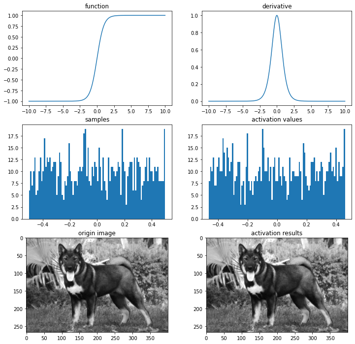
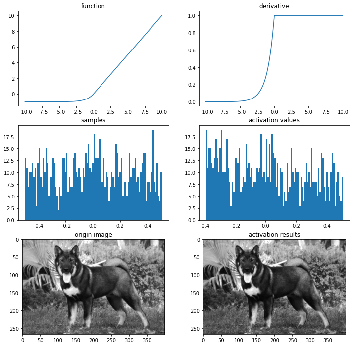
hyperbolic tangent

Solves the problem of not being zero centered but still has the vanishing gradient problem

하이퍼볼릭 탄젠트 함수는 그래프에서도 알 수 있듯 -1 또는 1에서 포화됩니다.

import os
img_path = os.getenv('HOME')+'/aiffel/activation/jindo_dog.jpg'

# 하이퍼볼릭 탄젠트 함수
def tanh(x):
    return (np.exp(x)-np.exp(-x))/(np.exp(x)+np.exp(-x))

def dev_tanh(x):
    return 1-tanh(x)**2

# 시각화
ax = plot_and_visulize(img_path, tanh, dev_tanh)
ax.show()

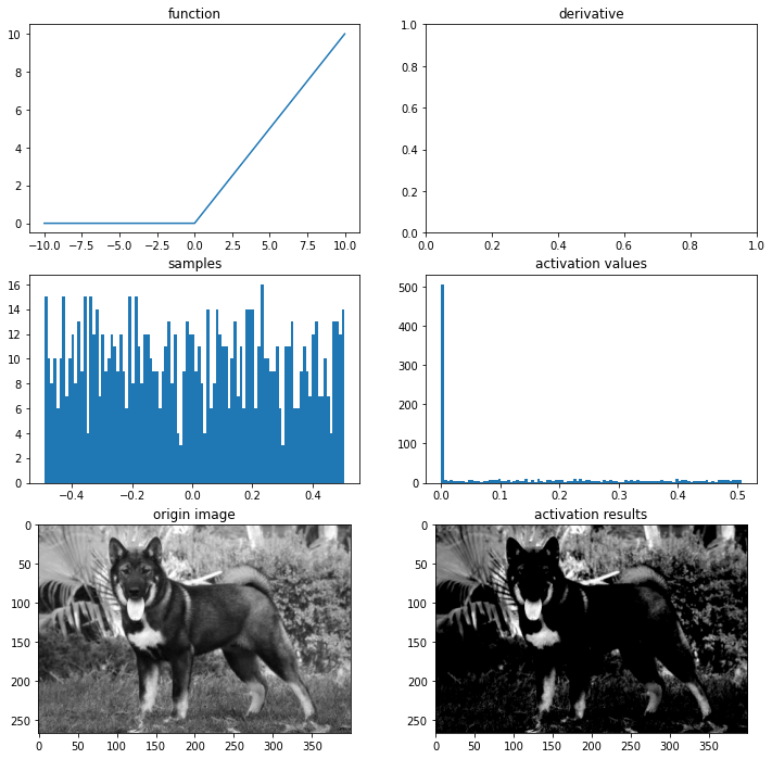
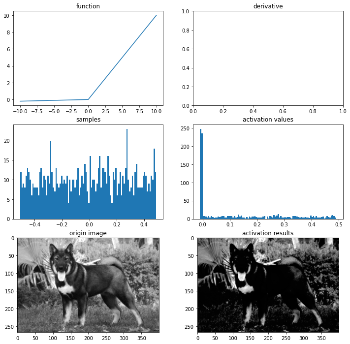
ReLU

import os
img_path = os.getenv('HOME')+'/aiffel/activation/jindo_dog.jpg'

# relu 함수
def relu(x):
    return max(0,x)

# 시각화
ax = plot_and_visulize(img_path, relu)
ax.show()

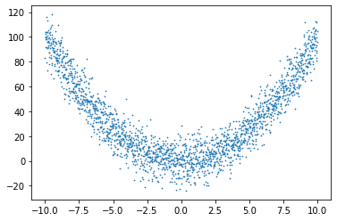
q_X = np.array([-10+x/100 for x in range(2001)])
q_y = np.array([(x)**2 + np.random.randn(1)*10 for x in q_X])
plt.scatter(q_X, q_y, s=0.5)

<matplotlib.collections.PathCollection at 0x7fa8f4463790>

approx_relu_model_p = tf.keras.Sequential([
    tf.keras.layers.Input(shape=(1,)),
    tf.keras.layers.Dense(6, activation='relu'), # 6 nodes 병렬 연결
    tf.keras.layers.Dense(1)
])
approx_relu_model_p.compile(loss='mse', optimizer=tf.keras.optimizers.Adam(learning_rate=0.005), metrics=['accuracy'])
approx_relu_model_p.fit(q_X, q_y, batch_size=32, epochs=100, verbose=0)

approx_relu_model_s = tf.keras.Sequential([
    tf.keras.layers.Input(shape=(1,)),
    tf.keras.layers.Dense(2, activation='relu'),# 2 nodes 직렬로 3번 연결
    tf.keras.layers.Dense(2, activation='relu'),
    tf.keras.layers.Dense(2, activation='relu'),
    tf.keras.layers.Dense(1)
])
approx_relu_model_s.compile(loss='mse', optimizer=tf.keras.optimizers.Adam(learning_rate=0.005), metrics=['accuracy'])
approx_relu_model_s.fit(q_X, q_y, batch_size=32, epochs=100, verbose=0)

approx_relu_model_p.summary()
approx_relu_model_s.summary()

Model: "sequential_10"
_________________________________________________________________
Layer (type)                 Output Shape              Param #   
=================================================================
dense_11 (Dense)             (None, 6)                 12        
_________________________________________________________________
dense_12 (Dense)             (None, 1)                 7         
=================================================================
Total params: 19
Trainable params: 19
Non-trainable params: 0
_________________________________________________________________
Model: "sequential_11"
_________________________________________________________________
Layer (type)                 Output Shape              Param #   
=================================================================
dense_13 (Dense)             (None, 2)                 4         
_________________________________________________________________
dense_14 (Dense)             (None, 2)                 6         
_________________________________________________________________
dense_15 (Dense)             (None, 2)                 6         
_________________________________________________________________
dense_16 (Dense)             (None, 1)                 3         
=================================================================
Total params: 19
Trainable params: 19
Non-trainable params: 0
_________________________________________________________________

q_test_X = q_X.reshape((*q_X.shape,1))
plt.figure(figsize=(10,5))

ax1 = plt.subplot(1,2,1)
ax1.set_title('parallel')
pred_y_p = approx_relu_model_p(q_test_X)
ax1.plot(q_X, pred_y_p)

ax2 = plt.subplot(1,2,2)
ax2.set_title('serial')
pred_y_s = approx_relu_model_s(q_test_X)
ax2.plot(q_X, pred_y_s)

plt.show()

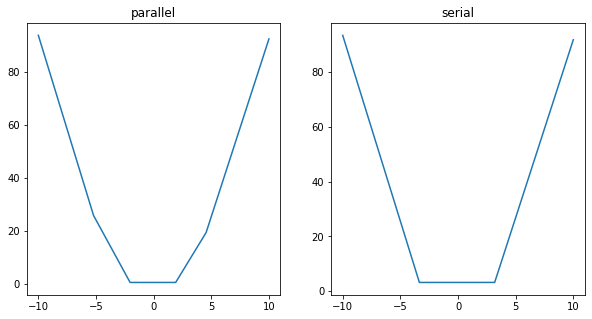
파라미터 수가 같음에도 불구하고 노드를 병렬로 쌓은 것이 직렬로 쌓은 것보다 더 좋은 결과를 낸 것을 확인할 수 있었습니다.

disadvantages of ReLU

ReLU 함수의 출력값이 00이 중심이 아닙니다. 따라서 위에서 언급햇던 문제가 발생할 수 있습니다.

또 하나의 단점은 Dying ReLU입니다. 즉, 이 노드의 출력값과 그래디언트가 0이 되어 노드가 죽어버립니다. 이러한 문제는 특히 학습률(learning rate)을 크게 잡을 때 자주 발생합니다. 반대로 학습률을 줄여준다면 이 문제는 적게 발생합니다.

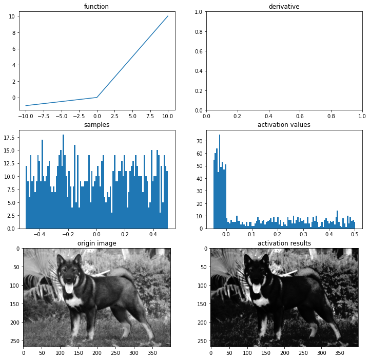
Leaky ReLU

import os
img_path = os.getenv('HOME')+'/aiffel/activation/jindo_dog.jpg'

# leaky relu 함수
def leaky_relu(x):
    return max(0.02*x,x)

# 시각화
ax = plot_and_visulize(img_path, leaky_relu)
ax.show()

PReLU

# PReLU 함수
def prelu(x, alpha):
    return max(alpha*x,x)

# 시각화
ax = plot_and_visulize(img_path, lambda x: prelu(x, 0.1)) # parameter alpha=0.1일 때

ax.show()

ELU

# ELU 함수
def elu(x, alpha):
    return x if x > 0 else alpha*(np.exp(x)-1)

def dev_elu(x, alpha):
    return 1 if x > 0 else elu(x, alpha) + alpha

# 시각화
ax = plot_and_visulize(img_path, lambda x: elu(x, 1), lambda x: dev_elu(x, 1)) # alpha가 1일 때
ax.show()